CV for the Exclusive Lasso
cv.exclusive_lasso(
  X,
  y,
  groups,
  ...,
  family = c("gaussian", "binomial", "poisson"),
  offset = rep(0, NROW(X)),
  weights = rep(1, NROW(X)),
  type.measure = c("mse", "deviance", "class", "auc", "mae"),
  nfolds = 10,
  parallel = FALSE
)

# S3 method for ExclusiveLassoFit_cv
plot(x, bar.width = 0.01, ...)
Arguments
| X | The matrix of predictors (\(X \in \R^{n \times p}\)) |
|---|---|
| y | The response vector (\(y\)) |
| groups | An integer vector of length \(p\) indicating group membership.
(Cf. the |
| ... | Additional arguments passed to |
| family | The GLM response type. (Cf. the |
| offset | A vector of length \(n\) included in the linear predictor. |
| weights | Weights applied to individual
observations. If not supplied, all observations will be equally
weighted. Will be re-scaled to sum to \(n\) if
necessary. (Cf. the |
| type.measure | The loss function to be used for cross-validation. |
| nfolds | The number of folds (\(K\)) to be used for K-fold CV |
| parallel | Should CV run in parallel? If a parallel back-end for the
|
| x | An |
| bar.width | Width of error bars |
Details
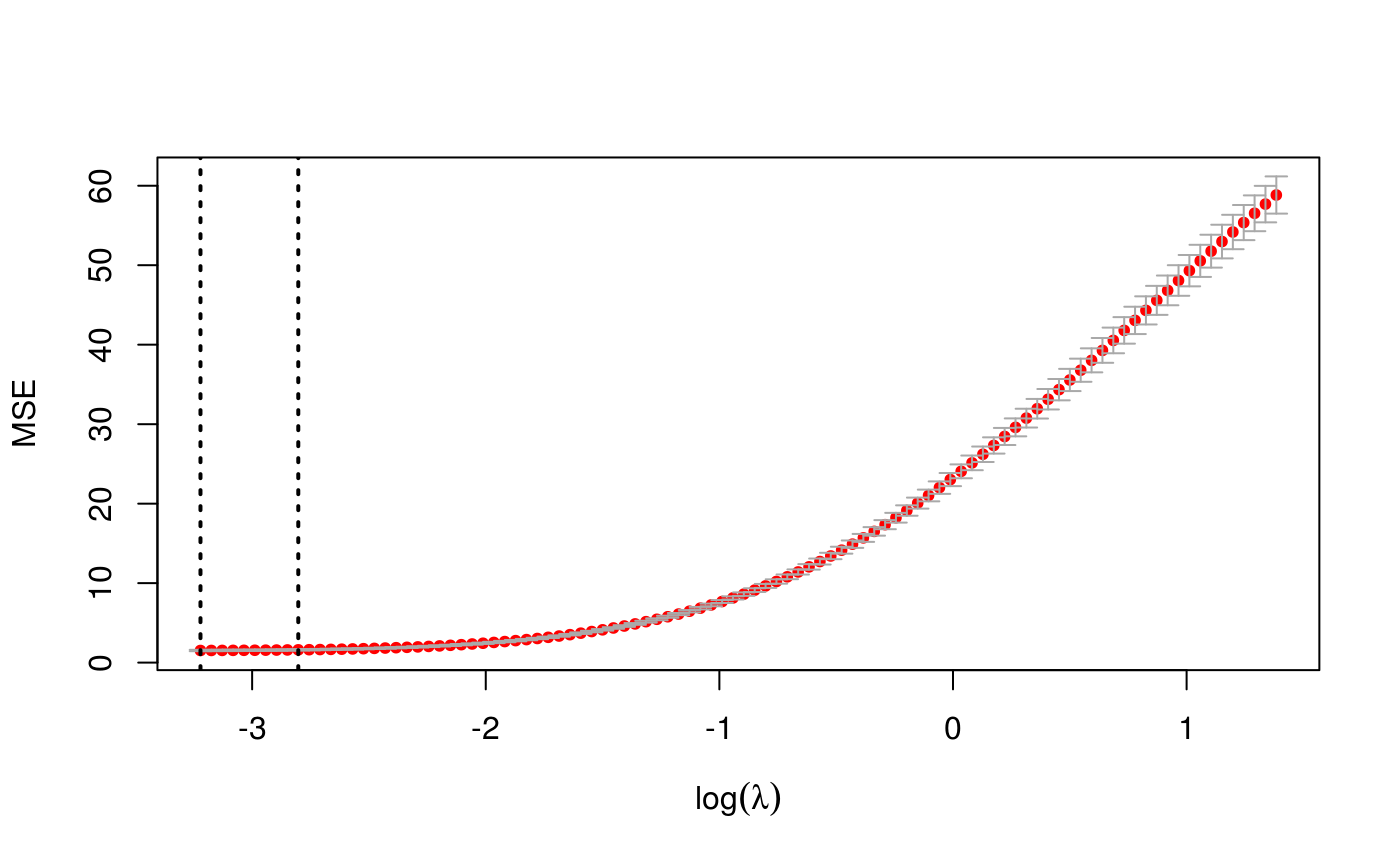
As discussed in Appendix F of Campbell and Allen [1], cross-validation can be quite unstable for exclusive lasso problems. Model selection by BIC or EBIC tends to perform better in practice.
References
Campbell, Frederick and Genevera I. Allen. "Within Group Variable Selection with the Exclusive Lasso." Electronic Journal of Statistics 11(2), pp.4220-4257. 2017. doi: 10.1214/EJS-1317
Examples
n <- 200 p <- 500 groups <- rep(1:10, times=50) beta <- numeric(p); beta[1:10] <- 3 X <- matrix(rnorm(n * p), ncol=p) y <- X %*% beta + rnorm(n) exfit_cv <- cv.exclusive_lasso(X, y, groups, nfolds=5) print(exfit_cv)#> Exclusive Lasso CV #> ------------------ #> #> Lambda (Min Rule): 0.03990931 #> Lambda (1SE Rule): 0.06065861 #> #> Loss Function: mse #> #> Time: 6.252 secs #> #> Full Data Fit #> ------------- #> Exclusive Lasso Fit #> ------------------- #> #> N: 200. P: 500. #> 10 groups. Median size 50 #> #> Grid: 100 values of lambda. #> Miniumum: 0.03990931 #> Maximum: 3.990931 #> Degrees of freedom: 1.933574 --> 50.92902 #> Number of selected variables: 10 --> 53 #> #> Fit Options: #> - Family: Gaussian #> - Intercept: TRUE #> - Standardize X: TRUE #> - Algorithm: Coordinate Descent #> #> Time: 1.018 secs #>plot(exfit_cv)# coef() and predict() work just like # corresponding methods for exclusive_lasso() # but can also specify lambda="lambda.min" or "lambda.1se" coef(exfit_cv, lambda="lambda.1se")#> 501 x 1 sparse Matrix of class "dgCMatrix" #> #> (Intercept) -0.0077801499 #> 2.6822769050 #> 2.8165965650 #> 2.8518035316 #> 2.6544234540 #> 2.8677254880 #> 2.8478057952 #> 2.8090797152 #> 2.7992287242 #> 2.8086392724 #> 2.5816691772 #> . #> . #> . #> . #> . #> . #> . #> . #> . #> . #> . #> . #> . #> . #> . #> . #> . #> . #> . #> . #> . #> . #> . #> . #> . #> . #> . #> . #> . #> . #> . #> . #> . #> . #> . #> . #> . #> . #> . #> . #> . #> . #> . #> . #> . #> . #> . #> . #> . #> . #> . #> . #> . #> . #> . #> . #> . #> . #> . #> . #> . #> . #> . #> . #> . #> . #> . #> . #> . #> . #> . #> . #> . #> . #> . #> . #> . #> . #> . #> . #> . #> . #> . #> -0.0098949880 #> . #> . #> . #> . #> . #> 0.0165309113 #> . #> . #> . #> . #> . #> . #> . #> . #> . #> . #> . #> . #> . #> . #> . #> . #> . #> . #> . #> . #> . #> . #> . #> . #> . #> . #> . #> . #> . #> . #> . #> . #> . #> . #> . #> . #> . #> . #> . #> . #> . #> . #> . #> . #> . #> . #> . #> . #> . #> . #> . #> . #> . #> . #> . #> . #> . #> . #> . #> . #> 0.0006515005 #> . #> . #> . #> . #> . #> . #> . #> . #> . #> . #> . #> . #> . #> . #> . #> . #> . #> . #> . #> . #> . #> . #> . #> . #> . #> . #> . #> . #> . #> . #> . #> . #> . #> . #> . #> . #> 0.0635293515 #> . #> . #> . #> . #> . #> -0.0078353797 #> . #> . #> . #> . #> . #> . #> . #> . #> . #> . #> . #> . #> . #> . #> . #> . #> . #> . #> . #> . #> . #> . #> . #> . #> . #> 0.0064978996 #> . #> . #> . #> . #> . #> . #> . #> 0.0656433933 #> . #> . #> . #> . #> . #> . #> . #> . #> . #> . #> . #> . #> . #> . #> . #> . #> . #> . #> . #> . #> . #> . #> . #> . #> . #> 0.0189304398 #> . #> . #> . #> . #> . #> . #> . #> . #> . #> . #> . #> . #> . #> . #> . #> . #> . #> . #> . #> . #> . #> . #> . #> 0.0302486144 #> . #> . #> . #> . #> . #> . #> . #> . #> . #> . #> . #> . #> . #> . #> . #> . #> . #> . #> . #> . #> . #> . #> . #> . #> . #> . #> . #> . #> . #> . #> . #> . #> . #> . #> . #> . #> . #> . #> . #> . #> 0.0205647162 #> . #> . #> . #> . #> . #> . #> . #> . #> . #> . #> . #> . #> . #> . #> . #> . #> . #> . #> . #> 0.1159623435 #> . #> . #> . #> . #> . #> . #> . #> . #> . #> . #> . #> . #> . #> . #> . #> . #> . #> 0.0017285968 #> . #> . #> . #> . #> . #> . #> . #> . #> -0.0201977863 #> 0.0161054123 #> . #> . #> . #> . #> . #> . #> . #> . #> . #> . #> . #> . #> . #> . #> . #> . #> . #> . #> . #> . #> . #> . #> . #> . #> . #> . #> . #> . #> . #> . #> . #> . #> . #> . #> . #> . #> . #> . #> . #> . #> . #> . #> . #> . #> . #> . #> . #> -0.0274158940 #> . #> . #> . #> . #> . #> . #> . #> . #> . #> . #> . #> . #> . #> . #> . #> . #> . #> . #> . #> . #> . #> . #> . #> . #> . #> . #> . #> . #> . #> . #> . #> . #> . #> . #> . #> . #> . #> . #> . #> . #> . #> . #> . #> . #> . #> . #> . #> . #> -0.0221223490 #> . #> . #> 0.0097299240 #> . #> . #> . #> . #> . #> . #> . #> . #> . #> . #> . #> . #> . #> . #> . #> . #> . #> . #> . #> . #> . #> . #> .