10-Minute Introduction to ClustRviz
Michael Weylandt
Department of Statistics, Rice Universitymichael.weylandt@rice.edu
John Nagorski
Department of Statistics, Rice UniversityGenevera I. Allen
Jan and Dan Duncan Neurological Research Institute, Baylor College of Medicine
gallen@rice.edu
Last Updated: August 19th, 2020
Source:vignettes/Tutorial.Rmd
Tutorial.RmdIntroduction
The clustRviz package intends to make fitting and visualizing CARP and CBASS solution paths an easy process. In the QuickStart vignette we provide a quick start guide for basic usage, fitting, and plotting. In this vignette, we build on the basics and provide a more detailed explanation for the variety of options available in clustRviz.
Background
The starting point for CARP is the Convex Clustering (Hocking et al. 2011; Chi and Lange 2015; Tan and Witten 2015) problem:
\[\text{arg min}_{U} \frac{1}{2}\|U - X\|_F^2 + \lambda\sum_{(i, j) \in \mathcal{E}} w_{ij} \|U_{i\cdot} - U_{j\cdot}\|_q\]
where \(X\) is an \(n \times p\) data matrix, consisting of \(p\) measurements on \(n\) subjects, \(\lambda \in \mathbb{R}_{> 0}\) a regularization parameter determining the degree of clustering, and \(w_{ij}>0\) a weight for each pair of observations; here \(\| . \|_F\) and \(\| . \|_2\) denote the Frobenius norm and \(\ell_q\) norm, respectively. (Typically, we take \(q = 2\).)
Briefly, Convex Clustering seeks to find and estimate a matrix \(\hat{U} \in \mathbb{R}^{n\times p}\) which is both faithful to the original data (Frobenius norm loss term) and has columns “shrunk” together by the fusion penalty term. The penalty term induces “clusters” of equal columns in \(U\) - if the difference is zero, then the columns must be equal - while still maintaining closeness to the original data. The equal columns of \(U\) can then be used to assign clusters among the columns of \(X\).
Unlike other clustering parameters, \(\lambda\) can be varied smoothly. At one end, for zero or very small \(\lambda\), the fusion penalty has minimal effect and all the columns of \(\hat{U}\) are distinct, implying \(n\) different (trivial) clusters. At the other end, for large \(\lambda\), all columns of \(U\) are fused together into a single “mono-cluster.” Between these extremes, every other degree of clustering can be found as \(\lambda\) varies. Considered as a function of \(\lambda\), the columns of \(\hat{U}_{\lambda}\) form continuous paths, which we will visualize below.
To solve the Convex Clustering problem, Chi and Lange (2015) proposed to use the Alternating Direction Method of Multipliers (ADMM) (Boyd et al. 2011), an iterative optimization scheme. This performs well for a single value of \(\lambda\), but can become very expensive if we wish to investigate enough values of \(\lambda\) to form a (near-continuous) solution path. To address this, we adapt the Algorithmic Regularization framework proposed by Hu et al. (2016): this framework takes a single ADMM step, followed by a small increase in \(\lambda\). Remarkably, if the increases in \(\lambda\) are sufficiently small, it turns out that we can approximate the true solution path in a fraction of the time needed for full optimization. Additionally, because we consider a fine grid of \(\lambda\) values, we are able to get a much more accurate sense of the structure of the solution paths. This approach is called Clustering via Algorithmic Regularization Paths or CARP and is implemented in the function of the same name.
This tutorial will focus on convex clustering though the clustRviz package also provides functionality for convex biclustering via the Convex Biclustering via Algorithmic Regularization with Small Steps or CBASS algorithm, which combines algorithmic regularization with the Generalized ADMM proposed by Weylandt (2020). All of the graphics and data manipulation functionality demonstrated below for the CARP function work equally well for the CBASS function.
Data Preparation and Weight Calculation
While the CARP and CBASS functions provides several reasonable default choices for weights, algorithms, etc, it is important to know their details if one wishes to compute more customized clustering choices. Here we examine several of the inputs to CARP in more detail.
Here we use a dataset of presidential speechs obtained from The American Presidency Project to illustrate the use of clustRviz. The presidential speech data set contains the top 75 most variable log-transformed word counts of each US president, aggregated over several speeches. Additional text processing such as removing stop words and stemming have been done via the tm package.
Let’s begin by loading our package and the dataset:
library(clustRviz) data("presidential_speech") presidential_speech[1:5, 1:5] #> amount appropri british cent commerci #> Abraham Lincoln 3.433987 2.397895 1.791759 2.564949 2.708050 #> Andrew Jackson 4.248495 4.663439 2.995732 1.945910 3.828641 #> Andrew Johnson 4.025352 3.091042 2.833213 3.332205 2.772589 #> Barack Obama 1.386294 0.000000 0.000000 1.386294 0.000000 #> Benjamin Harrison 4.060443 4.174387 2.302585 4.304065 3.663562
As can be seen above, this data already comes to us as a data matrix with row and column labels. This is the best format to provide data to CARP, though if labels are missing, default labels will be automatically created.
Pre-Processing
An important first choice before clustering is whether to center and scale our observations. Column-wise centering is typically appropriate and is done by default, though this can be changed with the X.center argument. The matter of scaling is a bit more delicate and depends on whether the features are in some way directly comparable, in which case the raw scale may be meaningful, or are fundamentally incompatible, in which case it may make sense to remove scale effects. Scaling is controlled by the X.scale argument to CARP and is not implemented for CBASS. If scaling is requested, it is performed by the scale function from base R which performs unbiased (\(n-1\)) scaling. In the case of the presidental speech dataset, all variables are of the same type and so we will not scale our data matrix.
Clustering Weights
The choice of clustering weights \(w_{ij}\) is essential to getting reasonable clustering performance. CARP uses a reasonably robust heuristic that balances statistical and computational performance, but great improvements can be obtained by using bespoke weighting schemes. CARP allows weights to be specified as either a function which returns a weight matrix or a matrix of weights. More details are available in the Weights vignette
Dimension Reduction and Feature Selection
Convex clustering, as implemented in clustRviz, relies on the Euclidean distance (Frobenius norm) between points. As such, it is rather sensitive to “noisy” features. To achieve good performance in high-dimensional (big \(p\)) problems, it is often necessary to aggressively filter features or perform some sort of dimension reduction before clustering. Future versions of clustRviz will implement the sparse convex clustering method of Wang et al (2018) and the GeCCO+ scheme of Wang and Allen (2019), both of which allow for automatic feature weighting and selection.
clustRviz plots leading principal components by default in visualizations, though this is configurable. Note that the principal components projection is performed at fit time, not at plot time, so if higher principal components are desired, it may be necessary to increase the npcs argument to CARP.
Fitting
clustRviz aims to make it easy to compute the CARP and CBASS solution paths, and to quickly begin exploring the results. For now, we will use the defaults described above to cluster the presidential speech data via the CARP function:
carp_fit <- CARP(presidential_speech)
Once completed, we can examine a brief summary of the fitted object:
carp_fit #> CARP Fit Summary #> ==================== #> #> Algorithm: CARP (t = 1.05) #> Fit Time: 0.444 secs #> Total Time: 1.740 secs #> #> Number of Observations: 44 #> Number of Variables: 75 #> #> Pre-processing options: #> - Columnwise centering: TRUE #> - Columnwise scaling: FALSE #> #> Weights: #> - Source: Radial Basis Function Kernel Weights #> - Distance Metric: Euclidean #> - Scale parameter (phi): 0.01 [Data-Driven] #> - Sparsified: 4 Nearest Neighbors [Data-Driven]
The default output gives several useful pieces of information, including:
- the sample size (\(n = 44\)) and number of features in our data (\(p = 75\));
- the amount of time necessary to fit the cluster path (approximately 4 seconds);
- the preprocessing performed (centering, but not scaling); and
- the weighting scheme used:
- Radial Basis Function Kernel Weights based on the Euclidean Distance
- A scale parameter \(\phi = 0.01\) selected to maximize weight informativeness
- A high degree of sparsification (four nearest neighbors) to improve computation.
Each of these can be changed using parameters already discussed. Additionally, the printed output shows the step-size parameter \(t\) (default, used here, of 1.05). This means that at each iteration, \(\lambda\) is increased by 5%. For finer path approximations, the user can use a smaller value of \(t\), though be warned that this increases both computation time and memory usage.
CARP has three additional flags that control optimizer behavior:
-
norm(default2): should an \(\ell_2\) or \(\ell_1\) fusion penalty be used? The \(\ell_2\) penalty is rotationally symmetric and plays well with downstream principal components visualization, so it is used by default. -
exact(defaultFALSE): if this is set, the algorithmic regularization scheme is replaced with an exact optimization approach. This is often much more expensive, but guarantees exact solutions when they matter. -
back_track(defaultFALSE): in almost all settings, the monotonic increase of \(\lambda\) is sufficient to recover the structure of the convex clustering dendrogram. For pathological cases where the dendrogram is not easily recovered, enabling back-tracking will causeCARPto use a back-tracking bisection search to precisely identify when observations are fused together.
More advanced optimizer controls can be set using the clustRviz_options function.
Accessing Clustering Solutions
Once fit, the clustering solution may be examined via three related “accessor” functions:
-
get_cluster_labels: to get a named factor vector of cluster labels -
get_cluster_centroids: to get a matrix of cluster centroids -
get_clustered_data: to get the clustered data matrix (data replaced by estimated centroids)
The interface for these functions is essentially the same for CARP and CBASS objects, though the exact meaning of “centroids” varies between the problems (vectors for CARP and scalars for CBASS). The latter two functions also support a refit flag, which determines whether the convex clustering centroids or the naive centroids (based only on the convex clustering labels) are returned.
For example, we can extract the clustering labels from our carp_fit corresponding to a \(k = 2\) cluster solution:
cluster_labels <- get_cluster_labels(carp_fit, k = 2) head(cluster_labels) #> Abraham Lincoln Andrew Jackson Andrew Johnson Barack Obama #> cluster_1 cluster_1 cluster_1 cluster_2 #> Benjamin Harrison Calvin Coolidge #> cluster_1 cluster_1 #> Levels: cluster_1 cluster_2
We see a rather inbalanced data set (the “pre-WWII” cluster is much larger):
table(cluster_labels) #> cluster_labels #> cluster_1 cluster_2 #> 30 14
Similarly, to get the cluster means, we use the get_cluster_centroids function:
get_cluster_centroids(carp_fit, k = 2) #> amount appropri british cent commerci commission consider #> [1,] 3.247043 3.226682 2.3124551 2.0551206 2.7439237 2.3802731 3.63590 #> [2,] 1.862722 2.042501 0.5157932 0.7925161 0.9780746 0.1980421 1.46525 #> develop expenditur farm feder fiscal help indian #> [1,] 2.337113 3.088539 1.191574 2.378937 2.430556 0.9302646 2.772808 #> [2,] 3.715357 1.996894 2.392863 4.032946 2.582249 4.3600998 1.028310 #> intercours island june mail mexico navi need #> [1,] 2.346998 2.2486963 2.207865 2.0366255 2.4085862 2.8553629 2.610077 #> [2,] 0.000000 0.9483649 1.273441 0.4409847 0.7222947 0.9645195 4.444242 #> per provis receipt reform regard report shall subject #> [1,] 2.053577 3.316586 2.4005575 1.573253 2.881303 3.188971 3.873702 3.873460 #> [2,] 1.529186 1.351412 0.7369229 2.950234 1.399618 2.504706 2.266559 1.660877 #> territori treasuri treati upon vessel america bank incom #> [1,] 3.207658 3.270253 3.474962 4.470278 2.8743947 2.114410 2.464109 1.341383 #> [2,] 1.031974 1.170382 1.850235 2.707913 0.5064341 4.545829 1.961930 3.339435 #> million price spain articl cut dollar econom #> [1,] 1.794258 2.081976 1.9433860 2.3807624 0.7759532 1.480457 1.646237 #> [2,] 4.044070 3.083916 0.1980421 0.2475526 3.1468759 3.273746 3.999372 #> women educ school bill tariff unemploy weapon #> [1,] 0.5921557 1.902443 1.312848 1.870695 1.9435594 0.4278973 0.2676695 #> [2,] 2.9420389 3.463114 3.235803 2.843507 0.8874667 2.7956399 2.7877462 #> get method farmer challeng achiev democraci area #> [1,] 0.5174374 1.509951 1.134142 0.3849688 1.060422 0.3436318 0.9664067 #> [2,] 3.0255971 1.461203 2.349569 3.1210443 3.403615 2.5199520 3.0214103 #> billion problem basic budget goal job level #> [1,] 0.2822107 1.241074 0.1439163 0.4619983 0.1229626 0.1425555 0.5467032 #> [2,] 3.7429589 3.659555 2.8387802 3.7959956 3.2118895 3.9587172 3.0683132 #> nuclear percent program spend technolog today tonight #> [1,] 0.000000 0.1476939 0.4781129 0.2886231 0.02310491 0.3258551 0.000000 #> [2,] 2.559875 3.4095268 4.4328005 3.1180550 2.68228351 3.7233467 2.596381 #> worker inflat soviet #> [1,] 0.3094282 0.3914679 0.000000 #> [2,] 3.1347856 2.5319042 2.493221
Since we performed convex clustering here, our centroids are \(p\)-vectors. By default, the naive centroids are used; if we prefer the exact convex clustering solution, we can pass the refit = FALSE flag:
get_cluster_centroids(carp_fit, k = 2, refit = FALSE) #> amount appropri british cent commerci commission consider #> [1,] 3.155728 3.148065 2.1953481 1.9647108 2.622744 2.2361246 3.489258 #> [2,] 2.058397 2.210968 0.7667368 0.9862515 1.237746 0.5069316 1.779483 #> develop expenditur farm feder fiscal help indian #> [1,] 2.424643 3.012971 1.266860 2.483571 2.437900 1.152671 2.659366 #> [2,] 3.527792 2.158826 2.231534 3.808730 2.566511 3.883514 1.271401 #> intercours island june mail mexico navi need #> [1,] 2.1935090 2.161143 2.144818 1.9284549 2.2943682 2.729938 2.726907 #> [2,] 0.3289057 1.135979 1.408541 0.6727789 0.9670476 1.233286 4.193891 #> per provis receipt reform regard report shall subject #> [1,] 2.011753 3.183595 2.2906826 1.661924 2.784559 3.138733 3.765006 3.728682 #> [2,] 1.618809 1.636394 0.9723691 2.760226 1.606927 2.612360 2.499479 1.971115 #> territori treasuri treati upon vessel america bank incom #> [1,] 3.061643 3.128592 3.365123 4.350888 2.7191839 2.269599 2.428955 1.472401 #> [2,] 1.344863 1.473940 2.085605 2.963748 0.8390288 4.213282 2.037260 3.058681 #> million price spain articl cut dollar econom women #> [1,] 1.939146 2.144216 1.828425 2.2402022 0.9309466 1.597334 1.796562 0.7461207 #> [2,] 3.733596 2.950544 0.444386 0.5487529 2.8147471 3.023297 3.677248 2.6121139 #> educ school bill tariff unemploy weapon get method #> [1,] 2.002487 1.436163 1.933006 1.866371 0.5819261 0.4351889 0.6825409 1.502273 #> [2,] 3.248734 2.971558 2.709984 1.052870 2.4655782 2.4287760 2.6718040 1.477654 #> farmer challeng achiev democraci area billion problem basic #> [1,] 1.209656 0.5636847 1.213491 0.4858199 1.100357 0.509604 1.393858 0.3210233 #> [2,] 2.187753 2.7380816 3.075610 2.2152632 2.734374 3.255688 3.332161 2.4592651 #> budget goal job level nuclear percent program #> [1,] 0.6806464 0.3271903 0.3964664 0.7113691 0.1704463 0.3647129 0.7365316 #> [2,] 3.3274639 2.7742589 3.4146225 2.7154577 2.1946333 2.9444860 3.8790462 #> spend technolog today tonight worker inflat soviet #> [1,] 0.4756603 0.2001397 0.5470925 0.1728774 0.4958418 0.5305127 0.1660077 #> [2,] 2.7172610 2.3029232 3.2492666 2.2259298 2.7353280 2.2339511 2.1374900
We can instead supply the percent argument to specify \(\lambda\) (or more precisely, \(\lambda / \lambda_{\text{max}}\)) rather than the numer of clusters explicitly. For example, if we are interested at the clustering solution about \(25\%\) of the way along the regularization path:
get_cluster_labels(carp_fit, percent = 0.25) #> Abraham Lincoln Andrew Jackson Andrew Johnson #> cluster_1 cluster_1 cluster_1 #> Barack Obama Benjamin Harrison Calvin Coolidge #> cluster_2 cluster_1 cluster_1 #> Chester A. Arthur Donald J. Trump Dwight D. Eisenhower #> cluster_1 cluster_2 cluster_2 #> Franklin D. Roosevelt Franklin Pierce George Bush #> cluster_2 cluster_1 cluster_2 #> George W. Bush George Washington Gerald R. Ford #> cluster_2 cluster_1 cluster_2 #> Grover Cleveland Harry S. Truman Herbert Hoover #> cluster_1 cluster_2 cluster_1 #> James A. Garfield James Buchanan James K. Polk #> cluster_1 cluster_1 cluster_1 #> James Madison James Monroe Jimmy Carter #> cluster_1 cluster_1 cluster_2 #> John Adams John F. Kennedy John Quincy Adams #> cluster_1 cluster_2 cluster_1 #> John Tyler Lyndon B. Johnson Martin van Buren #> cluster_1 cluster_2 cluster_1 #> Millard Fillmore Richard Nixon Ronald Reagan #> cluster_1 cluster_2 cluster_2 #> Rutherford B. Hayes Theodore Roosevelt Thomas Jefferson #> cluster_1 cluster_1 cluster_1 #> Ulysses S. Grant Warren G. Harding William Henry Harrison #> cluster_1 cluster_3 cluster_1 #> William Howard Taft William J. Clinton William McKinley #> cluster_1 cluster_2 cluster_1 #> Woodrow Wilson Zachary Taylor #> cluster_1 cluster_1 #> Levels: cluster_1 cluster_2 cluster_3
We see that our data is clearly falls into three clusters.
Simiarly to CARP objects, CBASS clustering solutions may also be extracted via the three accessor functions. The CBASS methods allow one of three parameters to be used to specify the solution:
-
k.row: the number of row clusters -
k.col: the number of column clusters -
percent: the percent of total regularization
Other than this, the behavior of get_cluster_labels, and get_clustered_data is roughly the same:
# CBASS Cluster Labels for rows (observations = default) get_cluster_labels(cbass_fit, percent = 0.85, type = "row") # CBASS Cluster Labels for columns (features) get_cluster_labels(cbass_fit, percent = 0.85, type = "col") # CBASS Solution - naive centroids get_clustered_data(cbass_fit, percent = 0.85) # CBASS Solution - convex bi-clustering centroids get_clustered_data(cbass_fit, percent = 0.85, refit = FALSE)
The get_cluster_centroids function returns a \(k_1\)-by-\(k_2\) matrix, giving the (scalar) centroids at a solution with \(k_1\) row clusters and \(k_2\) column clusters:
get_cluster_centroids(cbass_fit, percent = 0.85)
Visualizations
clustRviz provides a rich set of visualization tools based on the ggplot2 and plotly libraries. Because clustRviz integrates with these libraries, it is easy to develop custom visualizations based on clustRviz defaults.
Path Plots
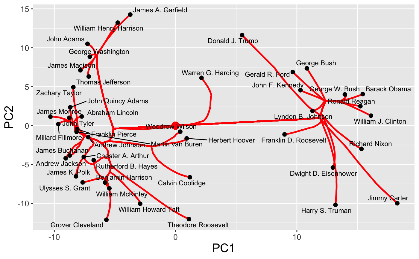
The first type of path supported by clustRviz is one obtained by plotting values of \(\hat{U}_{\lambda}\) for various values of \(\lambda\). Because \(\hat{U}\) is a continuous function of \(\lambda\), these paths are continuous and make for attractive visualizations. As mentioned above, clustRviz defaults to plotting the first two principal components of the data:
plot(carp_fit, type = "path")
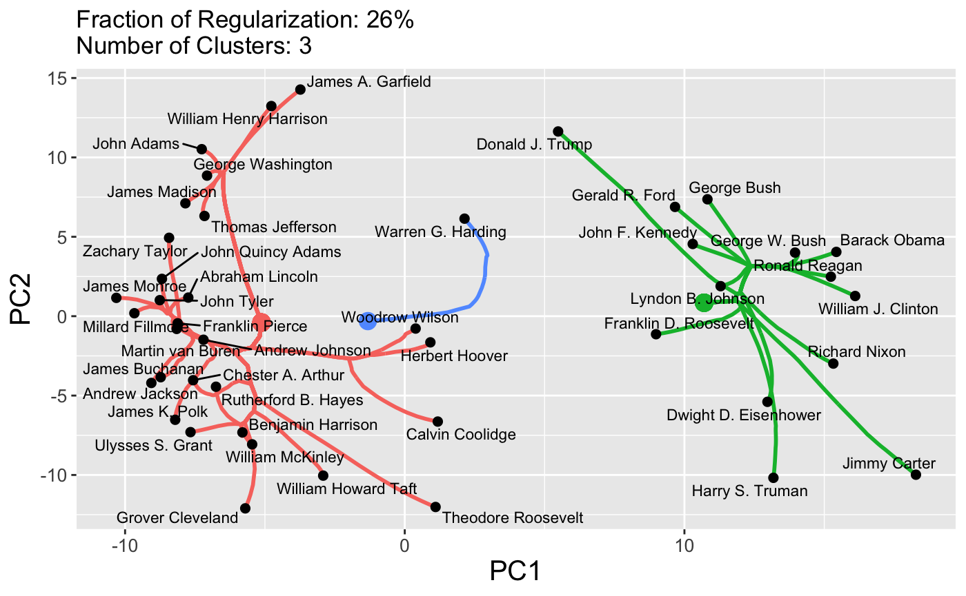
By default, the entire path is shown, but we can specify a number of clusters directly:
plot(carp_fit, type = "path", k = 3)
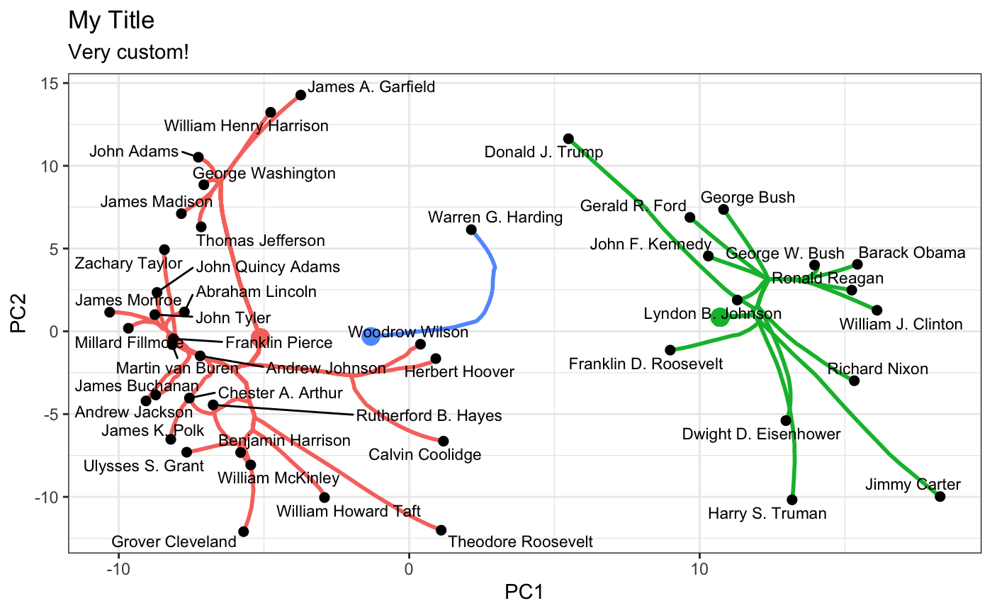
These plots are standard ggplot objects and can be customized in the usual manner:
plot(carp_fit, type = "path", k = 3) + ggplot2::theme_bw() + ggplot2::ggtitle("My Title", subtitle = "Very custom!")
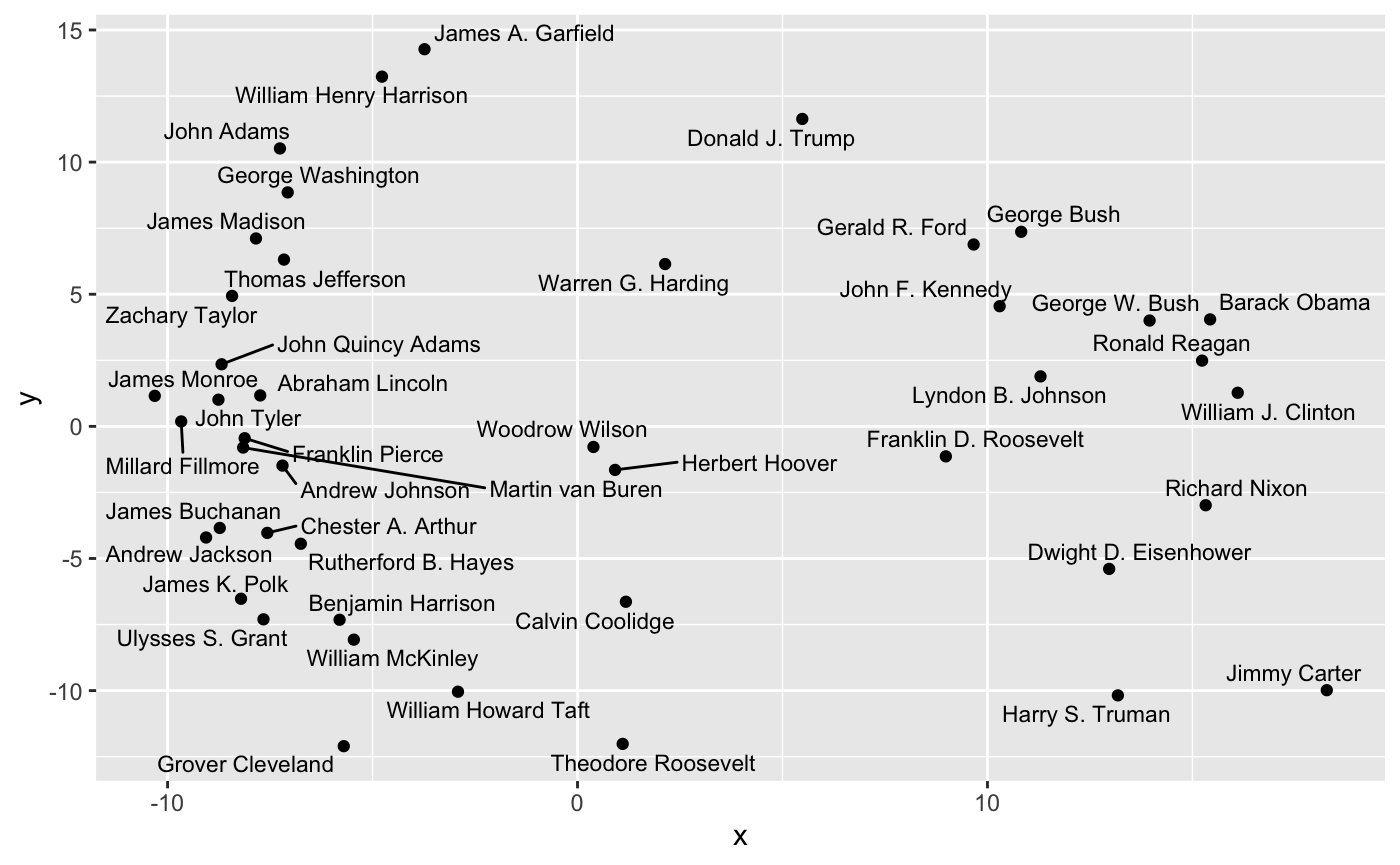
We can also plot the raw features directly:
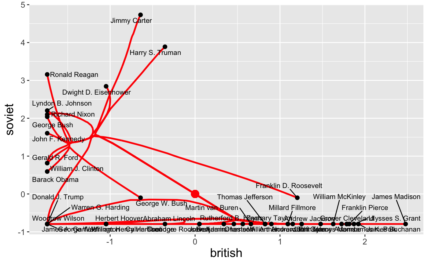
In this space, clear differences in pre-Cold War and post-Cold War topics of presidential speeches are evident. This sort of customized plot can be saved to a file using the standard ggplot2::ggsave functionality.
Because paths are continuous, it is also possible to set the dynamic = TRUE flag to produce a GIF via the gganimate package:
plot(carp_fit, type = "path", dynamic = TRUE)
Finally, interactive path plots can be produced using the plotly library by setting interactive = TRUE:
plot(carp_fit, type = "path", dynamic = TRUE, interactive = TRUE) #> Warning: `arrange_()` is deprecated as of dplyr 0.7.0. #> Please use `arrange()` instead. #> See vignette('programming') for more help #> This warning is displayed once every 8 hours. #> Call `lifecycle::last_warnings()` to see where this warning was generated. #> Warning: `group_by_()` is deprecated as of dplyr 0.7.0. #> Please use `group_by()` instead. #> See vignette('programming') for more help #> This warning is displayed once every 8 hours. #> Call `lifecycle::last_warnings()` to see where this warning was generated.