Finding Common Origins of Milky Way Stars

Author

Andersen Chang, Tiffany M. Tang, Tarek M. Zikry, Genevera I. Allen

Published

June 4, 2025

Fit Clustering Pipelines on Training Data

In this section, we detail our clustering pipeline.

Clustering Methods Under Study:

  • K-means Clustering
  • Hierarchical Clustering with Euclidean distance and either complete or Ward’s linkage
  • Spectral Clustering with nearest neighbors affinity and number of neighbors = 5, 30, 60, or 100

For each of these clustering methods, we examine the clustering results across different choices of the number of clusters \(k = 2, \ldots, 30\).

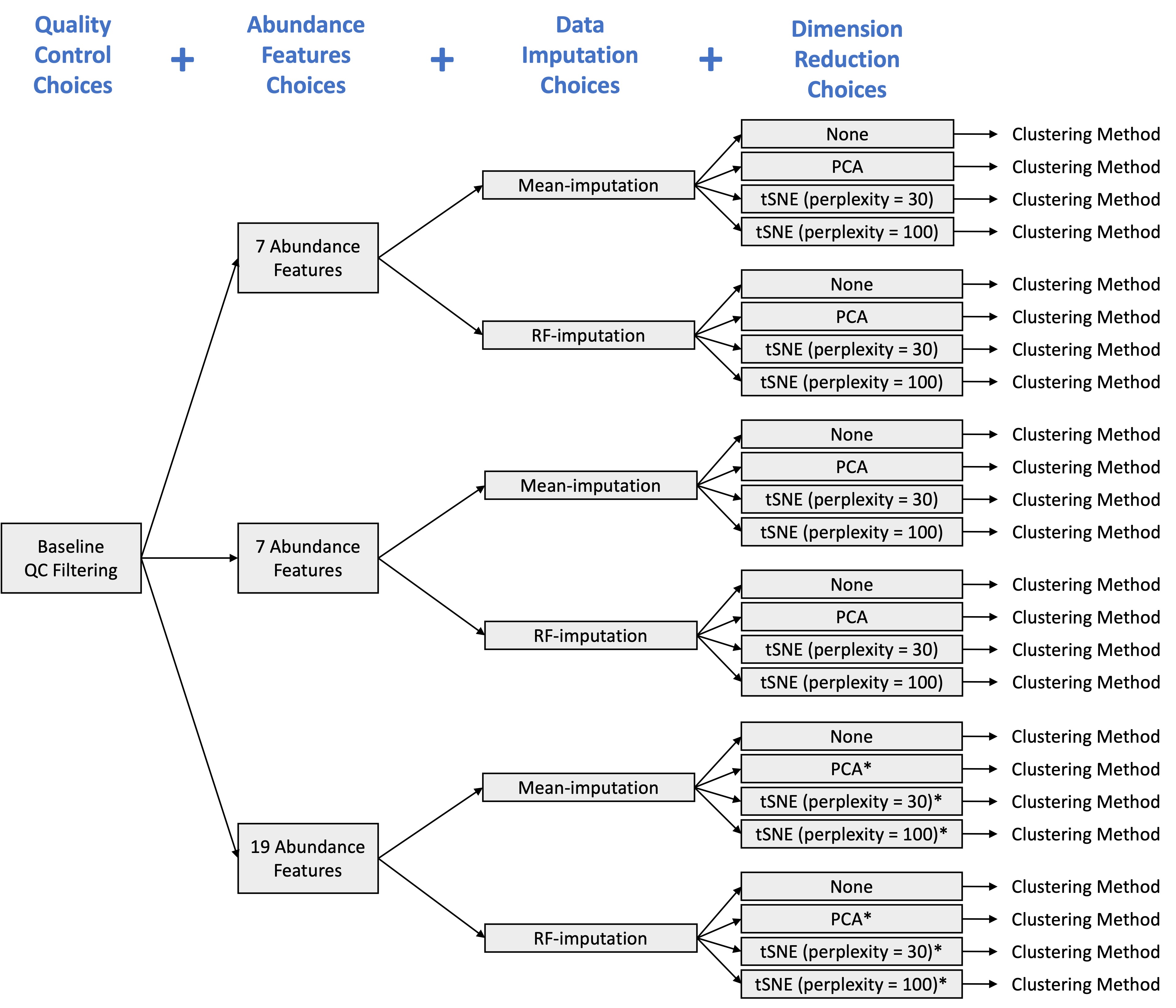
There are also many different ways one could apply these clustering methods. For example, one could apply it to the chemical abundance data directly or to a dimension-reduced version of the chemical abundance data. There are also other preprocessing choices, such as how to perform quality control filtering, which chemical abundance features are used, and how to impute missing data. In the figure below, we outline the various data preprocessing pipelines (prior to clustering) that are considered in this case study. Note that we only included the (tuned) dimension reduction methods that exhibited high neighborhood retention from the previous investigation (i.e., PCA, tSNE (perplexity = 30), and tSNE (perplexity = 100)), and for PCA, the top four components were chosen based on the scree plot. We will refer to the set of these data preprocessing pipelines as \(\mathcal{G}\).

Set of data preprocessing pipelines considered prior to applying clustering methods in case study. Pipelines marked with an astericks were excluded to reduce the computational burden; however, results are similar even when including these pipelines.

Set of data preprocessing pipelines considered prior to applying clustering methods in case study. Pipelines marked with an astericks were excluded to reduce the computational burden; however, results are similar even when including these pipelines.
Show Code to Fit Clustering Pipelines on Training Data
## this code chunk fits the clustering pipelines on the training data

#### choose imputation methods ####
data_ls <- list(
  "Mean-imputed" = data_mean_imputed$train,
  "RF-imputed" = data_rf_imputed$train
)

#### choose number of features ####
feature_modes <- list(
  "Small" = 7,
  "Medium" = 11,
  "Big" = 19
)

#### choose ks ####
ks <- 2:30

#### choose dimension reduction methods ####
# raw data
identity_fun_ls <- list("Raw" = function(x) x)

# pca
pca_fun_ls <- list("PCA" = purrr::partial(fit_pca, ndim = 4))

# tsne
tsne_perplexities <- c(30, 100)
tsne_fun_ls <- purrr::map(
  tsne_perplexities,
  ~ purrr::partial(fit_tsne, dims = 2, perplexity = .x)
) |> 
  setNames(sprintf("tSNE (perplexity = %d)", tsne_perplexities))

# putting it together
dr_fun_ls <- c(
  identity_fun_ls,
  pca_fun_ls,
  tsne_fun_ls
)

#### choose clustering methods ####
# kmeans
kmeans_fun_ls <- list("K-means" = purrr::partial(fit_kmeans, ks = ks))

# hierarchical clustering
hclust_params <- list(
  d = c("euclidean"),
  linkage = c("complete", "ward.D")
) |> 
  expand.grid()
hclust_fun_ls <- purrr::map(
  1:nrow(hclust_params),
  ~ purrr::partial(
    fit_hclust, 
    ks = ks,
    d = hclust_params$d[[.x]],
    linkage = hclust_params$linkage[[.x]]
  )
) |> 
  setNames(
    sprintf(
      "Hierarchical (dist = %s, link = %s)",
      hclust_params$d, hclust_params$linkage
    )
  )

# spectral clustering
n_neighbors <- c(5, 30, 60, 100)
spectral_fun_ls <- purrr::map(
  n_neighbors,
  ~ purrr::partial(
    fit_spectral_clustering, 
    ks = ks,
    affinity = "nearest_neighbors",
    n_neighbors = .x
  )
) |> 
  setNames(sprintf("Spectral (n_neighbors = %s)", n_neighbors))

# putting it together
clust_fun_ls <- c(
  kmeans_fun_ls,
  hclust_fun_ls,
  spectral_fun_ls
)

#### Fit Clustering Pipelines ####
pipe_tib <- tidyr::expand_grid(
  data = data_ls,
  feature_mode = feature_modes,
  dr_method = dr_fun_ls,
  clust_method = clust_fun_ls
) |> 
  dplyr::mutate(
    impute_mode_name = names(data),
    feature_mode_name = names(feature_mode),
    dr_method_name = names(dr_method),
    clust_method_name = names(clust_method),
    name = stringr::str_glue(
      "{clust_method_name} [{impute_mode_name} + {feature_mode_name} + {dr_method_name}]"
    )
  ) |> 
  # remove some clustering pipelines to reduce computation burden
  dplyr::filter(
    # remove all big feature set + dimension-reduction runs
    !((dr_method_name != "Raw") & (feature_mode_name == "Big"))
  )
pipe_ls <- split(pipe_tib, seq_len(nrow(pipe_tib))) |> 
  setNames(pipe_tib$name)

fit_results_fname <- file.path(RESULTS_PATH, "clustering_fits_train.rds")
if (!file.exists(fit_results_fname)) {
  library(future)
  plan(multisession, workers = NCORES)
  
  # fit clustering pipelines (if not already cached)
  clust_fit_ls <- furrr::future_map(
    pipe_ls,
    function(pipe_df) {
      g <- create_preprocessing_pipeline(
        feature_mode = pipe_df$feature_mode[[1]],
        preprocess_fun = pipe_df$dr_method[[1]]
      )
      clust_out <- pipe_df$clust_method[[1]](
        data = pipe_df$data[[1]], preprocess_fun = g
      )
      return(clust_out)
    },
    .options = furrr::furrr_options(
      seed = TRUE, 
      globals = list(
        ks = ks,
        create_preprocessing_pipeline = create_preprocessing_pipeline,
        get_abundance_data = get_abundance_data,
        tsne_perplexities = tsne_perplexities,
        hclust_params = hclust_params,
        n_neighbors = n_neighbors,
        fit_kmeans = fit_kmeans,
        fit_hclust = fit_hclust,
        fit_spectral_clustering = fit_spectral_clustering
      )
    )
  )
  # save fitted clustering pipelines
  saveRDS(clust_fit_ls, file = fit_results_fname)
} else {
  # read in fitted clustering pipelines (if already cached)
  clust_fit_ls <- readRDS(fit_results_fname)
}

To see and interact with the training clustering results, we have developed a shiny app, which can be run locally in R/RStudio by typing the following in your R console:

view_clusters_app()

Hyperparameter Tuning and Model Selection via Cluster Stability

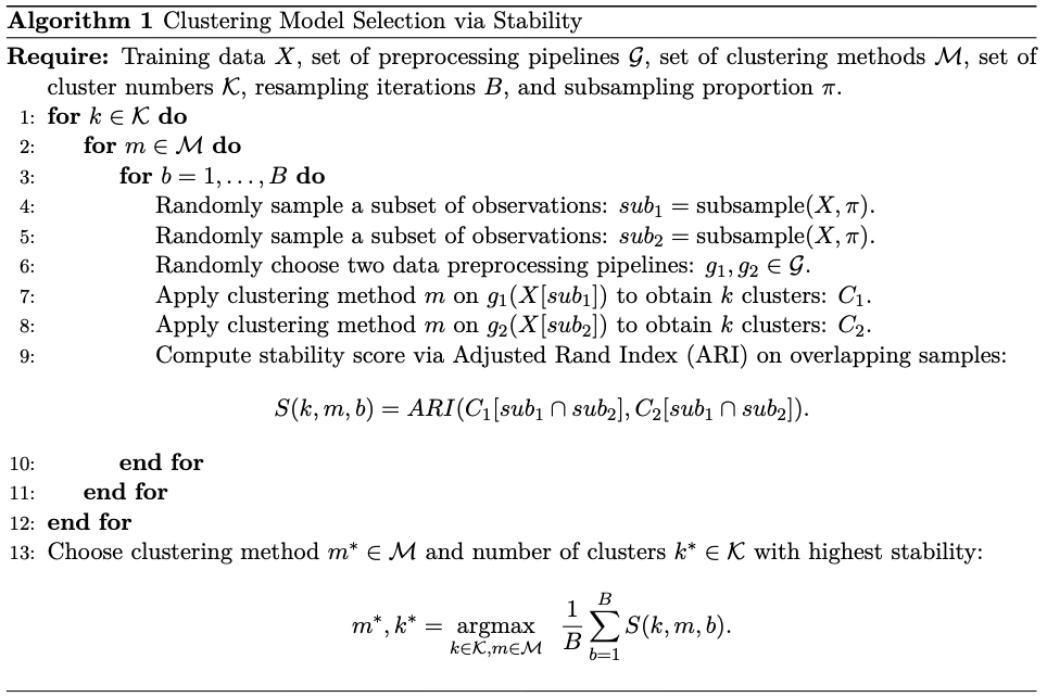
To select the best clustering method and number of clusters \(k\), we propose a stability-driven model selection procedure. Here, given our goal of working towards scientific discovery, we operate under the driving philosophy that our scientific conclusions should not be robust or stable across arbitrary human judgment calls such as the data preprocessing pipelines outlined in the above figure. Driven by this “stability principle”, we hence select the clustering method and number of clusters that yields the most stable (or similar) clustering results regardless of the data subsample used for training and regardless of the choice of data preprocessing pipeline \(g \in \mathcal{G}\). To operationalize this idea, we implement Algorithm 1 below, which is inspired by the Model Explorer algorithm from Ben-Hur, Elisseeff, and Guyon (2001).

Show Code to Tune/Evaluate Clustering Pipelines via Cluster Stability
## this code chunk performs model selection and hyperparameter tuning for the trained clustering pipelines

#### ModelExplorer hyperparameters ####
n_subsamples <- 50 # Number of subsamples
subsample_frac <- 0.8 # Proportion of data to subsample
max_pairs <- 100  # max num of pairs of subsamples to evaluate cluster stability
metric <- "ARI"  # metrics to compute for cluster stability

n <- nrow(data_ls$`Mean-imputed`)
fit_results_fname <- file.path(RESULTS_PATH, "clustering_subsampled_fits.rds")
stability_results_fname <- file.path(
  RESULTS_PATH, sprintf("clustering_subsampled_stability_%s.RData", metric)
)
if (!file.exists(fit_results_fname) ||
    !file.exists(stability_results_fname)) {
  library(future)
  plan(multisession, workers = NCORES)

  # fit clustering pipelines on subsampled data (if not already cached)
  clust_subsampled_fit_ls <- purrr::map(
    1:n_subsamples,
    function(b) {
      # get subsampled indices
      subsampled_idxs <- sort(
        sample(1:n, size = subsample_frac * n, replace = FALSE)
      )
      furrr::future_map(
        pipe_ls,
        function(pipe_df) {
          # fit clustering pipeline on subsample
          g <- create_preprocessing_pipeline(
            feature_mode = pipe_df$feature_mode[[1]],
            preprocess_fun = pipe_df$dr_method[[1]]
          )
          clust_out <- pipe_df$clust_method[[1]](
            data = pipe_df$data[[1]][subsampled_idxs, ], preprocess_fun = g
          )
          # return only the cluster ids for subsample
          cluster_ids <- purrr::map(
            clust_out$cluster_ids,
            function(cluster_ids) {
              out <- rep(NA, nrow(pipe_df$data[[1]]))
              out[subsampled_idxs] <- cluster_ids
              return(out)
            }
          )
          return(cluster_ids)
        },
        .options = furrr::furrr_options(
          seed = TRUE, 
          globals = list(
            ks = ks,
            subsampled_idxs = subsampled_idxs,
            create_preprocessing_pipeline = create_preprocessing_pipeline,
            get_abundance_data = get_abundance_data,
            tsne_perplexities = tsne_perplexities,
            hclust_params = hclust_params,
            n_neighbors = n_neighbors,
            fit_kmeans = fit_kmeans,
            fit_hclust = fit_hclust,
            fit_spectral_clustering = fit_spectral_clustering
          )
        )
      )
    }
  ) |> 
    setNames(as.character(1:n_subsamples)) |> 
    purrr::list_flatten(name_spec = "{inner} {outer}") |> 
    purrr::list_flatten(name_spec = "{inner}: {outer}")
  # save fitted clustering pipelines on subsampled data
  saveRDS(clust_subsampled_fit_ls, file = fit_results_fname)
  
  # create tibble of clustering results
  clusters_tib <- tibble::tibble(
    name = names(clust_subsampled_fit_ls),
    cluster_ids = clust_subsampled_fit_ls
  ) |> 
    annotate_clustering_results()
  
  # evaluate stability of clustering results per pipeline
  stability_per_pipeline <- clusters_tib |> 
    dplyr::group_by(
      k, pipeline_name, 
      impute_mode_name, feature_mode_name, dr_method_name, clust_method_name
    ) |>
    dplyr::summarise(
      cluster_list = list(cluster_ids),
      .groups = "drop"
    )
  stability_vals <- furrr::future_map(
    stability_per_pipeline$cluster_list,
    function(clusters) {
      cluster_stability(
        clusters, max_pairs = max_pairs, metrics = metric
      )[[metric]]
    },
    .options = furrr::furrr_options(
      seed = TRUE, 
      globals = list(
        cluster_stability = cluster_stability,
        max_pairs = max_pairs,
        metric = metric
      )
    )
  )
  stability_per_pipeline <- stability_per_pipeline |> 
    dplyr::mutate(
      group_name = pipeline_name,
      stability = !!stability_vals
    )
  
  # evaluate stability of clustering results per clustering method
  stability_per_clust_method <- clusters_tib |> 
    dplyr::group_by(
      k, clust_method_name
    ) |>
    dplyr::summarise(
      pipeline_names = list(unique(pipeline_name)),
      cluster_list = list(cluster_ids),
      .groups = "drop"
    )
  stability_vals <- furrr::future_map2(
    stability_per_clust_method$cluster_list,
    stability_per_clust_method$pipeline_names,
    function(clusters, pipe_names) {
      cluster_stability(
        clusters, max_pairs = max_pairs * length(pipe_names), metrics = metric
      )[[metric]]
    },
    .options = furrr::furrr_options(
      seed = TRUE, 
      globals = list(
        cluster_stability = cluster_stability,
        max_pairs = max_pairs,
        metric = metric
      )
    )
  )
  stability_per_clust_method <- stability_per_clust_method |>
    dplyr::mutate(
      group_name = clust_method_name,
      stability = !!stability_vals
    )
  
  save(
    stability_per_pipeline, 
    stability_per_clust_method, 
    file = stability_results_fname
  )
} else {
  # read in fitted clustering pipelines on subsampled data (if already cached)
  clust_subsampled_fit_ls <- readRDS(fit_results_fname)
  # read in evaluated stability of clustering results
  load(stability_results_fname)
}

The main results from our stability-driven model selection procedure are shown in the figure below under the Per Clustering Method tab.

Main Takeaways:

  • Spectral clustering (n_neighbors = 60) with \(k = 2\) clusters yields the most stable clusters
  • Interestingly, K-means with \(k = 8\) clusters also appears quite stable, considering that it is producing far more granular clusters than \(k = 2\).

Note: For completeness, the stability across subsamples per data preprocessing + clustering pipeline is provided under the Per Pipeline tab.

Stability of clustering pipelines across the number of clusters, measured via the adjusted Rand Index (ARI).

Stability of clustering pipelines across the number of clusters, measured via the adjusted Rand Index (ARI).

Estimate Consensus Clusters

For both Spectral Clustering (n_neighbors = 60) with \(k = 2\) clusters and K-means with \(k = 8\) clusters, we next aggregate the learned clusters across each of the data preprocessing pipelines using consensus clustering.

Show Code to Estimate Consensus Clusters
best_clust_methods <- list(
  "k = 2: Spectral (n_neighbors = 60)" = list(
    clust_method_name = "Spectral (n_neighbors = 60)",
    k = 2
  ),
  "k = 9: Spectral (n_neighbors = 60)" = list(
    clust_method_name = "Spectral (n_neighbors = 60)",
    k = 9
  ),
  "k = 8: K-means" = list(
    clust_method_name = "K-means", 
    k = 8
  )
)
clust_fit_ls <- purrr::map(clust_fit_ls, ~ .x$cluster_ids) |> 
  purrr::list_flatten(name_spec = "{inner}: {outer}")

consensus_clusters_results_path <- file.path(
  RESULTS_PATH, "consensus_clusters_train.rds"
)
consensus_nbhd_results_path <- file.path(
  RESULTS_PATH, "consensus_neighborhood_matrices_train.rds"
)
if (!file.exists(consensus_clusters_results_path) | 
    !file.exists(consensus_nbhd_results_path)) {
  nbhd_mat_ls <- list()
  consensus_out_ls <- list()
  for (i in 1:length(best_clust_methods)) {
    clust_method_name <- best_clust_methods[[i]]$clust_method_name
    k <- best_clust_methods[[i]]$k
    key <- names(best_clust_methods)[i]
    
    stable_clusters_tib_all <- tibble::tibble(
      name = names(clust_fit_ls),
      cluster_ids = clust_fit_ls
    ) |> 
      annotate_clustering_results() |> 
      dplyr::filter(
        k == !!k,
        clust_method_name == !!clust_method_name
      )
  
    keep_clust_ls <- stable_clusters_tib_all$cluster_ids
    # compute neighborhood matrix
    nbhd_mat_ls[[key]] <- get_consensus_neighborhood_matrix(keep_clust_ls)
    # aggregate stable clusters using consensus clustering
    consensus_out_ls[[key]] <- fit_consensus_clusters(nbhd_mat_ls[[key]], k = k)["cluster_ids"]
  }
  saveRDS(consensus_out_ls, file = consensus_clusters_results_path)
  saveRDS(nbhd_mat_ls, file = consensus_nbhd_results_path)
} else {
  # read in fitted clustering pipelines (if already cached)
  consensus_out_ls <- readRDS(consensus_clusters_results_path)
  nbhd_mat_ls <- readRDS(consensus_nbhd_results_path)
}

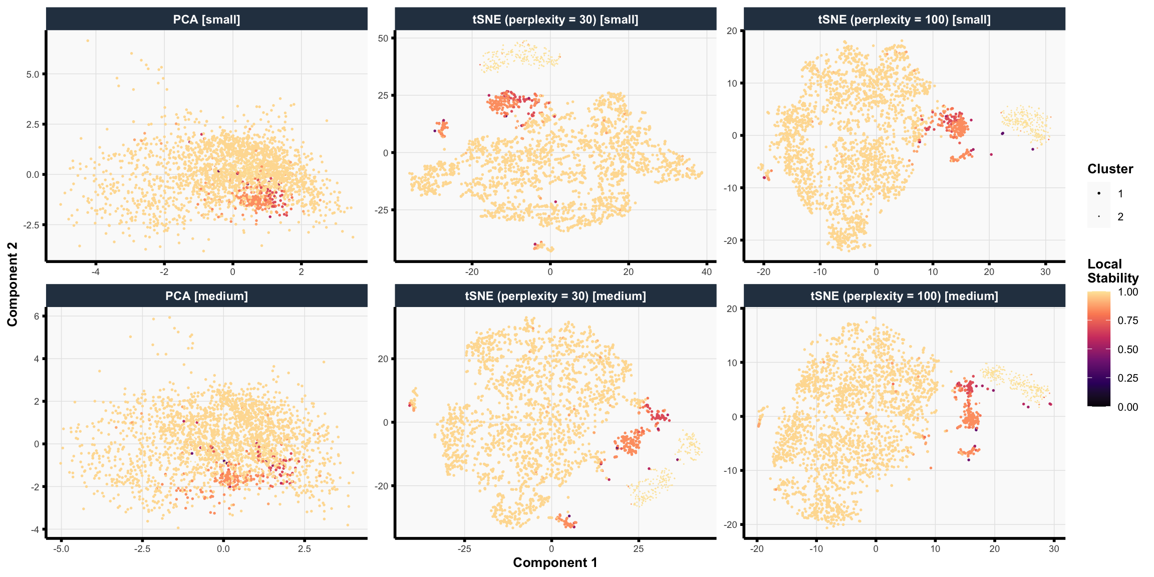
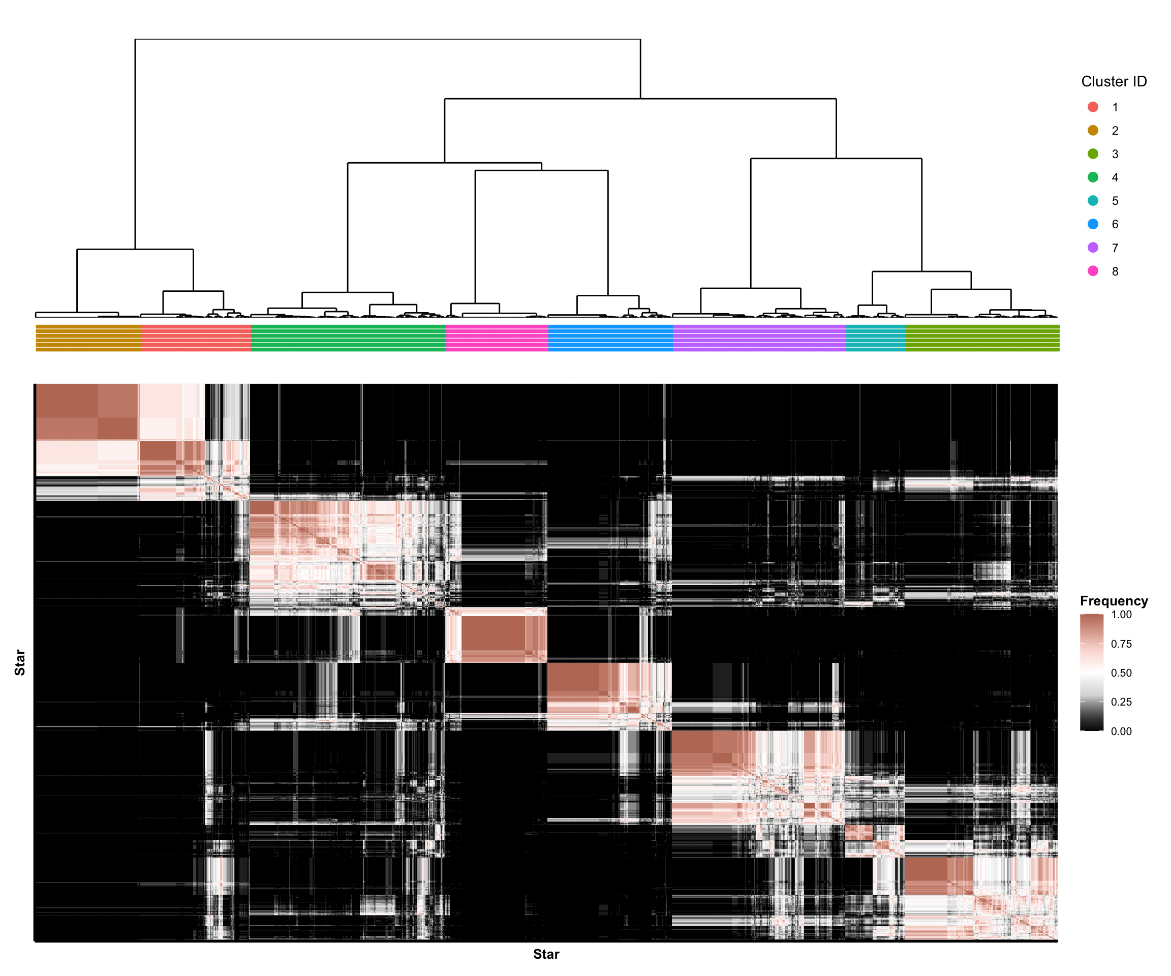
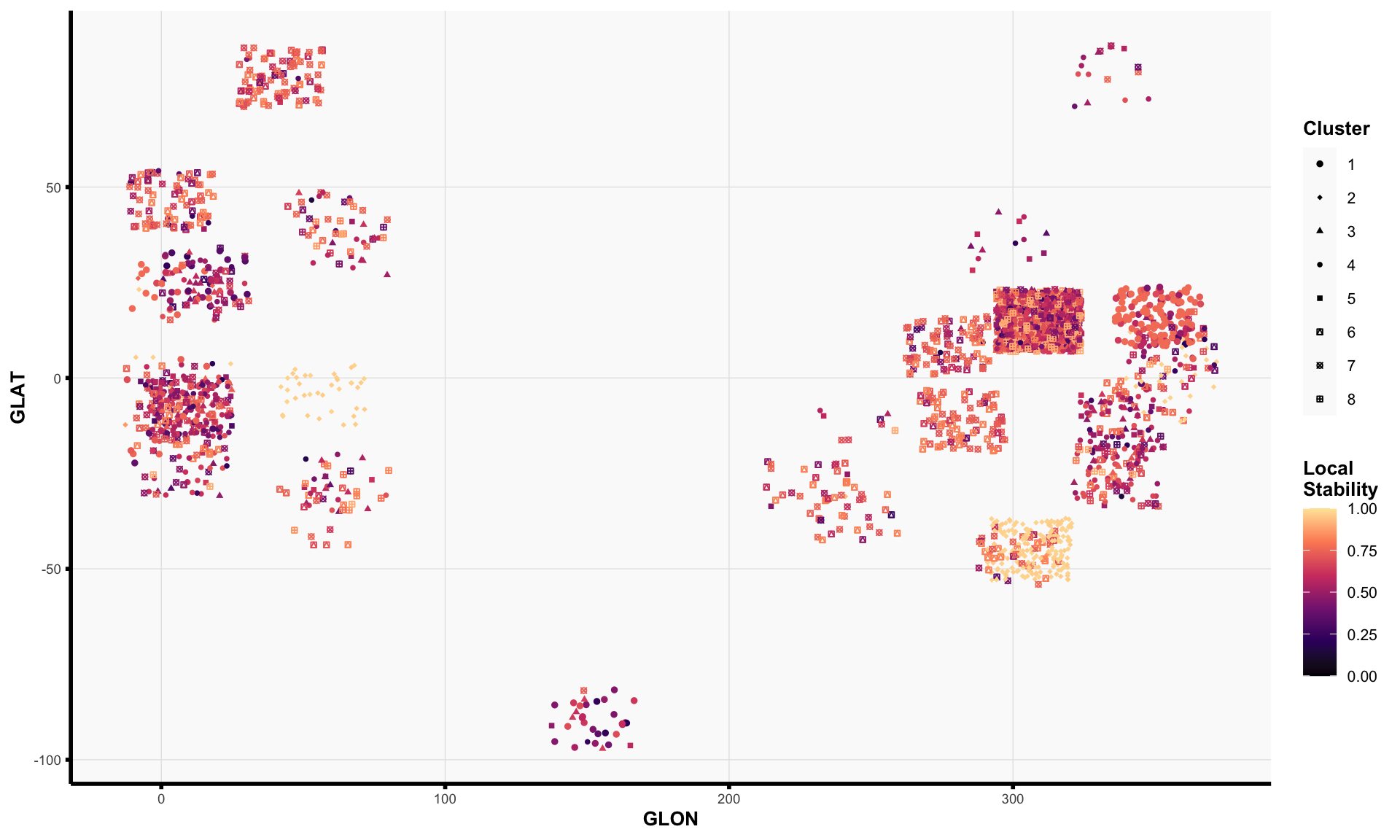
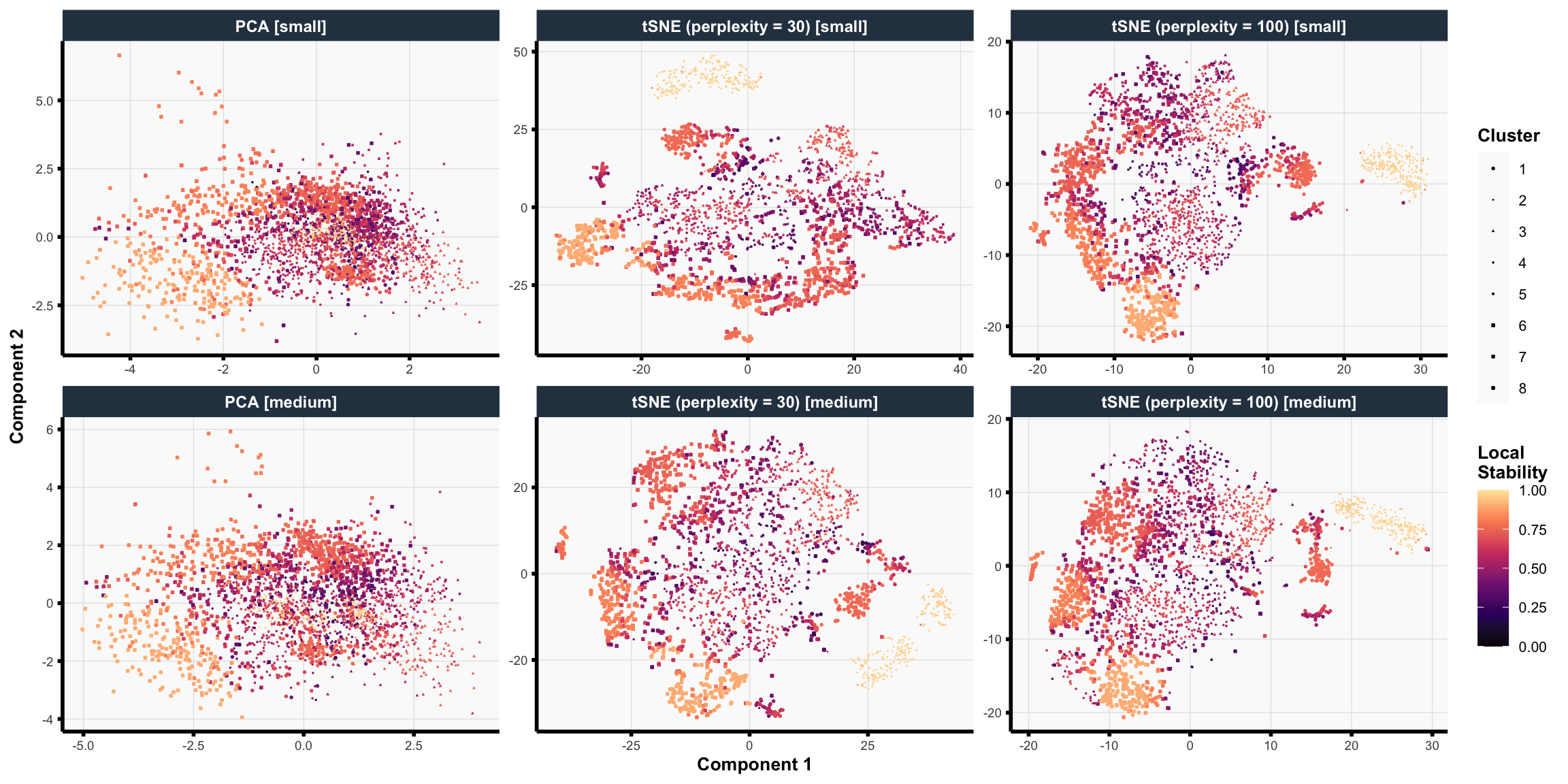
We visualize the resulting training consensus clusters in various ways below. Note:

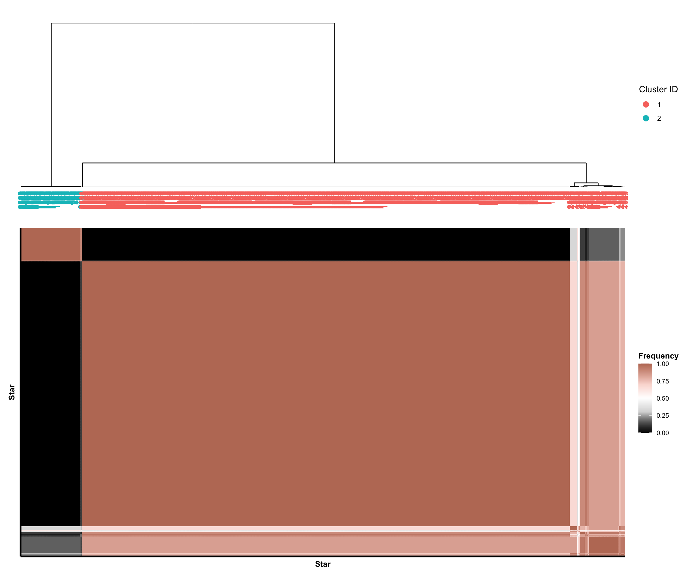
  • The frequencies shown in the consensus neighborhood heatmaps reveal the proportion of times that two stars were assigned to the same cluster across the different choices of data preprocessing pipelines.
    • High frequencies close to 1 indicate that the two stars were almost always in the same cluster.
    • Low frequencies close to 0 in the consensus neighborhood heatmaps indicate that the two stars were almost never in the same cluster.
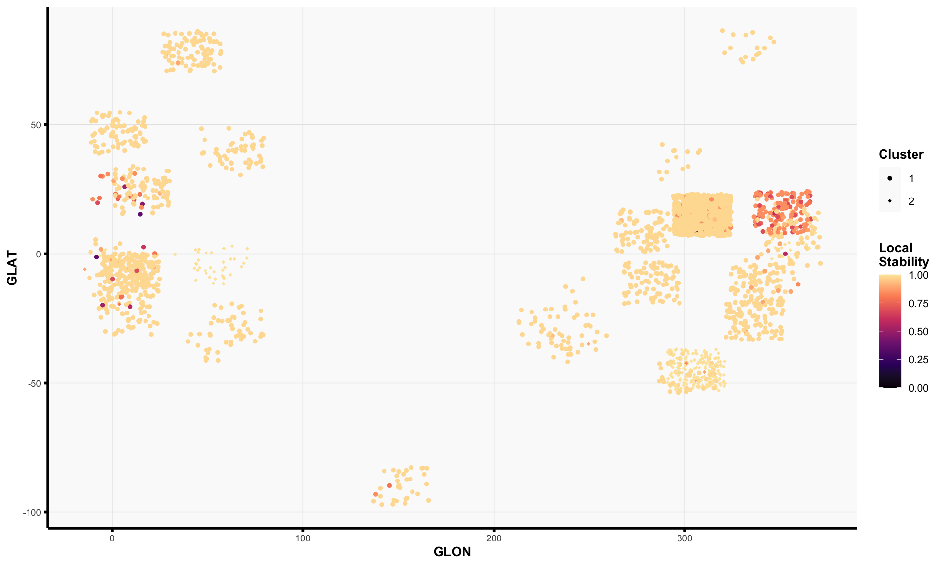
  • For each star, we define its local stability to be the average co-clustering frequency (i.e., the value shown in the consensus neighborhood heatmap) with all other stars in the same cluster. Intuitively, the local stability score for a star captures how consistently the star is clustered with other stars in its estimated cluster. Low local stability suggests that the star is not consistently clustered and may “hop” from one cluster to another depending on the data preprocessing choices.

Clearly, we observe that the two clusters from Spectral Clustering (n_neighbors = 60) are extremely stable; however, these two clusters largely recapitulate a well-known iron-rich versus iron-poor dichotomy between younger versus older stars in the Milky Way. Consequently, in an effort to seek new insights beyond this well-known phenomenon, we will turn our attention to the 8 clusters from K-means clustering for the remainder of this analysis.

Aside: What ifs…

In this section, we explore two hypothetical “what if” scenarios purely for didactic purposes.

First, what if we had chosen to use Spectral Clustering (n_neighbors = 60) with \(k = 9\) clusters, which yields a similar stability score as K-means with \(k = 8\) clusters?

In short, the clusters from Spectral Clustering (n_neighbors = 60) with \(k = 9\) clusters are quite similar to the that from K-means with \(k = 8\) clusters. This is most easily seen in the neighborhood heatmap below, which shows the co-cluster membership of each pair of stars. Red indicates that the two stars were in the same cluster in both clustering methods. Black indicates that the two stars were in different clusters in both clustering methods. White indicates that the two stars were in the same cluster in one clustering method but not the other.

Notably, cluster 2 from spectral clustering perfectly matches cluster 2 from K-means clustering. There is also very close alignment between several other clusters across methods, namely:

  • Spectral cluster 1 and K-means cluster 1
  • Spectral cluster 3 and K-means cluster 3
  • Spectral cluster 7 and K-means cluster 6
  • Spectral cluster 9 and K-means cluster 8

Furthermore, it appears that K-means cluster 4 is being split into two clusters by spectral clustering (clusters 4 and 6).

Neighborhood Heatmap

Consensus neighborhood heatmap between consensus clusters using Spectral (n_neighbors = 60) with k = 9 and K-means with k = 8.

Consensus neighborhood heatmap between consensus clusters using Spectral (n_neighbors = 60) with k = 9 and K-means with k = 8.

GCs per Cluster

Comparison of GC composition for each estimated consensus cluster.

Second, what if we had chosen to use only the most stable data preprocessing + clustering pipeline (i.e., K-means [Mean-imputed + Small + Raw]) instead of using the consensus across all data preprocessing pipelines?

The most stable data preprocessing + clustering pipeline choice is K-means, applied to the small feature set with mean-imputation and no dimension reduction prior to clustering. Applying this particular instantiation of K-means led to reasonable clusters, shown below. However, in the neighborhood heatmap, we observe an important difference between the consensus K-means pipeline (aggregated across all data preprocessing pipelines) versus the most stable K-means pipeline (using only the most stable data preprocessing choice) — that is, the most stable K-means pipeline grouped the consensus cluster 1 and consensus cluster 2 into a single cluster and created what appears to be a small and seemingly noisy cluster (“Most Stable Cluster 6”). Examining the GCs in each estimated cluster, we further see that the consensus K-means pipeline was able to separate two important GCs into distinct clusters — NGC6121 (dark green bar in cluster 1) and NGC0104 (orange bar in cluster 2) — while the most stable K-means pipeline grouped these two GCs into a single cluster. This is to show that the diversity of clusters across data preprocessing pipelines can help to improve the quality of the resulting clusters.

Neighborhood Heatmap

Consensus neighborhood heatmap between consensus clusters using K-means with k = 8, aggregated across all data preprocessing pipelines versus using only the most stable clustering pipeline.

Consensus neighborhood heatmap between consensus clusters using K-means with k = 8, aggregated across all data preprocessing pipelines versus using only the most stable clustering pipeline.

GCs per Cluster

Comparison of GC composition for each estimated consensus cluster.

References

Ben-Hur, Asa, Andre Elisseeff, and Isabelle Guyon. 2001. “A Stability Based Method for Discovering Structure in Clustered Data.” In Biocomputing 2002, 6–17. World Scientific.