Finding Common Origins of Milky Way Stars
Validation: Stability across Alternative Data Preprocessing
To begin validating the obtained (consensus) clusters from K-means with \(k = 8\) clusters, we assess the stability of the resulting clusters, had the same clustering pipeline been applied but with alternative data preprocessing choices. Importantly, we note that some data preprocessing choices (e.g., mean- versus RF-imputation, the set of chemical abundance features, and the dimension reduction method) have already been accounted for when performing the consensus clustering step discussed previously. However, due to the high computational burden, there are often more data preprocessing choices that are worth exploring than those that are feasible to include in the consensus step. For example, we have yet to investigate whether or not the resulting clusters are similar, had alternative quality control filtering thresholds been used.
Below, we repeat the clustering pipeline on the training data, but with alternative quality control filtering thresholds. Specifically, we marginally sweep across the following parameters:
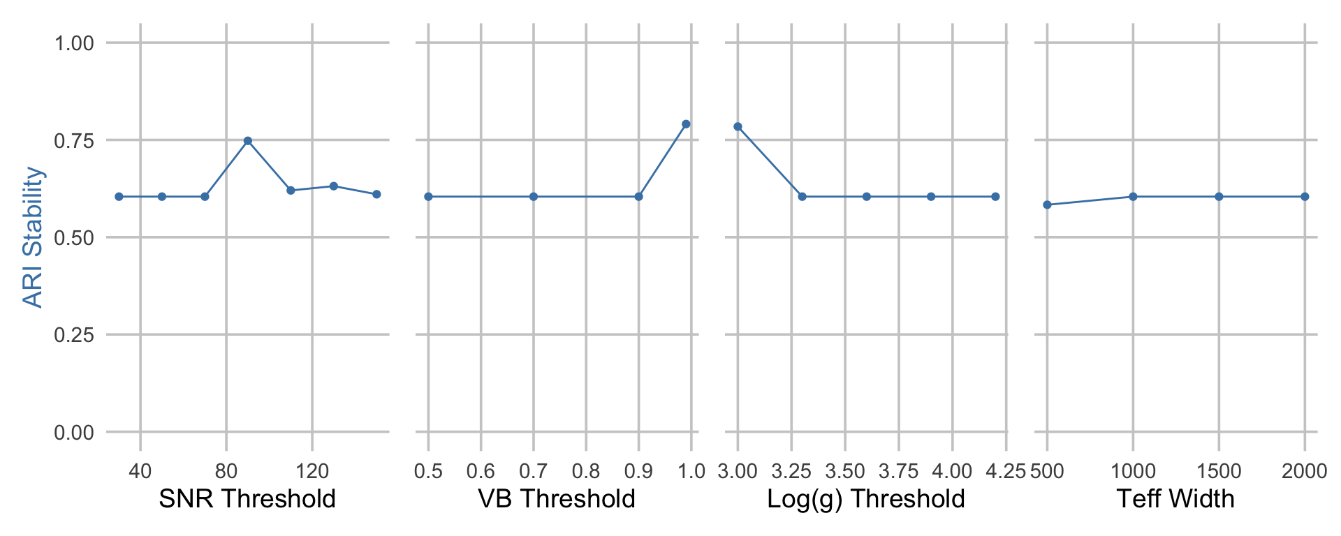
- Signal-to-noise (S/N) ratio threshold = 30, 50, 70\(^*\), 90, 110, 130, 150
- Effective temperature \(T_{eff}\) range width = 500, 1000\(^*\), 1500, 2000
- Logarithm of the surface gravity \(\log g\) = 3.0, 3.3, 3.6\(^*\), 3.9, 4.2
- GC membership probability = 0.5, 0.7, 0.9\(^*\), 0.99
We denote the default QC thresholds (used in previously in the main analysis) with an astericks (\(^*\)).
For each of these alternative choices, we compare the similarity between the original clusters and these new clusters using the adjusted Rand index (ARI). We report these results below. We find that the ARI at non-default filtering thresholds is both high and very similar to the ARI at the default filtering thresholds, indicating that the clusters are highly robust to these alternative data preprocessing choices.
Show Code to Evaluate Cluster Stability Across Alternative Data Preprocessing Pipelines
# Default QC thresholds
default_grid <- list(
  snr = 70,
  vb = 0.9,
  logg = 3.6,
  teff_width = 1000  # yields [3500, 5500]
)

# Parameter grids to sweep
vary_param_grid <- list(
  snr = c(30, 50, 70, 90, 110, 130, 150),
  vb = c(0.5, 0.7, 0.9, 0.99),
  logg = c(3.0, 3.3, 3.6, 3.9, 4.2),
  teff_width = c(500, 1000, 1500, 2000)
)

# Load data
data_mean_imputed_train <- dplyr::bind_cols(
  metadata$train, data_mean_imputed$train
)
data_rf_imputed_train <- dplyr::bind_cols(
  metadata$train, data_rf_imputed$train
)

# Get original cluster fit
orig_clusters <- readRDS(
  file.path(RESULTS_PATH, "consensus_clusters_train.rds")
)[[best_clust_method_name]]$cluster_ids

stability_results_fname <- file.path(
  RESULTS_PATH, "clustering_fits_stability.rds"
)

if (!file.exists(stability_results_fname)) {
  stability_fits_ls <- list()
  for (param_name in names(vary_param_grid)) {
    param_grid_ls <- default_grid
    param_grid_ls[[param_name]] <- vary_param_grid[[param_name]]
    param_grid <- expand.grid(param_grid_ls)
    stability_fits_ls[[param_name]] <- purrr::map(
      1:nrow(param_grid),
      function(i) {
        snr <- param_grid$snr[[i]]
        vb <- param_grid$vb[[i]]
        logg <- param_grid$logg[[i]]
        teff_width <- param_grid$teff_width[[i]]

        # get new QC-filtered data
        data_mean_imputed_qc <- apply_qc_filtering(
          data_mean_imputed_train,
          snr_threshold = snr,
          teff_thresholds = c(4500 - teff_width, 4500 + teff_width),
          logg_threshold = logg,
          starflag = 0,
          vb_threshold = vb
        )
        data_rf_imputed_qc <- apply_qc_filtering(
          data_rf_imputed_train,
          snr_threshold = snr,
          teff_thresholds = c(4500 - teff_width, 4500 + teff_width),
          logg_threshold = logg,
          starflag = 0,
          vb_threshold = vb
        )

        # get sample ids for new QC-filtered data
        keep_sample_idxs <- tibble::tibble(
          APOGEE_ID = data_mean_imputed_qc$meta$APOGEE_ID
        ) |>
          dplyr::left_join(
            dplyr::bind_cols(.id = 1:nrow(metadata$train), metadata$train),
            by = "APOGEE_ID"
          ) |>
          dplyr::pull(.id)

        # fit clustering pipeline on new QC-filtered data
        cluster_ids <- fit_best_pipeline(
          data_ls = list(
            "Mean-imputed" = data_mean_imputed_qc$abundance,
            "RF-imputed" = data_rf_imputed_qc$abundance
          ),
          k = best_k
        )

        # evaluate stability between original clusters and new clusters
        stability <- mclust::adjustedRandIndex(
          cluster_ids, orig_clusters[keep_sample_idxs]
        )

        return(list(
          sample_ids = keep_sample_idxs,
          cluster_ids = cluster_ids,
          stability = stability
        ))
      }
    ) |>
      setNames(vary_param_grid[[param_name]])
  }
  saveRDS(stability_fits_ls, stability_results_fname)
} else {
  stability_fits_ls <- readRDS(stability_results_fname)
}

stability_results_ls <- purrr::imap(
  stability_fits_ls,
  function(x, key) {
    purrr::map(x, ~ data.frame(stability = .x$stability)) |>
      dplyr::bind_rows(.id = key) |>
      dplyr::mutate(
        {{key}} := as.numeric(.data[[key]])
      )
  }
)

plt_ls <- purrr::imap(
  stability_results_ls,
  function(stability_df, key) {
    param_title <- dplyr::case_when(
      key == "snr" ~ "SNR Threshold",
      key == "vb" ~ "VB Threshold",
      key == "logg" ~ "Log(g) Threshold",
      key == "teff_width" ~ "Teff Width"
    )
    stability_df |>
      ggplot2::ggplot() +
      ggplot2::aes(x = !!rlang::sym(key), y = stability) +
      ggplot2::geom_line(width = 1.2, color = "steelblue") +
      ggplot2::geom_point(width = 2.5, color = "steelblue") +
      ggplot2::ylim(c(0, 1)) +
      ggplot2::labs(
        x = param_title,
        y = "ARI Stability",
      ) +
      ggplot2::theme_minimal(base_size = 14) +
      ggplot2::theme(
        panel.grid.major = ggplot2::element_line(color = "grey80"),
        panel.grid.minor = ggplot2::element_blank(),
        axis.title.y.left = ggplot2::element_text(color = "steelblue")
      )
  }
)

plt <- patchwork::wrap_plots(plt_ls, nrow = 1) +
  patchwork::plot_layout(axes = "collect")
subchunkify(
  plt, fig_height = 4, fig_width = 10,
  caption = "'Stability of cluster labels across different choices of data preprocessing pipelines.'"
)Validation: Cluster Generalizability
We next assess the overall generalizability of our estimated clusters using the held-out test set and the idea of cluster predictability. Specifically, we (i) apply the same consensus K-means with \(k = 8\) clustering pipeline to the training and test data separately, (ii) fit a random forest (RF) using the training covariates data to predict the cluster labels on the training set, (iii) use this trained RF to predict the cluster labels on the test set, and (iv) evaluate the concordance (via ARI) between the test cluster labels and the RF-predicted cluster labels on the test set. Note that this procedure relies on some preprocessed version of the covariates (i.e., abundance) data, and we thus report the generalizability using various data preprocessing pipelines below. In general, the choice of data preprocessing does not substantially impact the overall cluster generalizability, which is consistently between 0.39-0.43 ARI.
Though this ARI is not particularly high, there are select clusters that are far more generalizable than others. This can be seen by examining the confusion tables below (under the Confusion Tables tab). For example, the cluster labeled “Predicted 8” (i.e., cluster 8 from the training data) is highly generalizable and directly maps to cluster 7 in the test data. On the other hand, the cluster labeled “Predicted 3” (i.e., cluster 3 from the training data) is often confused with test clusters 2, 3 and 4.
To more rigorously quantify this cluster-specific notion of generalizability, we define a local generalizability metric, computed as the precision (i.e., TP/(TP + FP)) of each cluster. (Note: since the cluster labels are arbitrary, we align the RF-predicted clusters and the estimated test clusters based upon the pairing with the largest overlap and report the precision given that mapping.) These local generalizability scores clearly indicate that clusters 1, 2, 6, and 8 from the training dataset are highly predictable and generalizable while other clusters such as cluster 3 are less generalizable.
Show Code to Evaluate Cluster Generalizability using Test Data
## this code chunk evaluates cluster generalizability using test data

#### choose imputation methods ####
test_data_ls <- list(
  "Mean-imputed" = data_mean_imputed$test,
  "RF-imputed" = data_rf_imputed$test
)
train_data_ls <- list(
  "Mean-imputed" = data_mean_imputed$train,
  "RF-imputed" = data_rf_imputed$train
)

#### choose number of features ####
feature_modes <- list(
  "Small" = 7,
  "Medium" = 11,
  "Big" = 19
)

#### choose ks ####
ks <- c(2, 8, 9)

#### choose dimension reduction methods ####
# raw data
identity_fun_ls <- list("Raw" = function(x) x)

# pca
pca_fun_ls <- list("PCA" = purrr::partial(fit_pca, ndim = 4))

# tsne
tsne_perplexities <- c(30, 100)
tsne_fun_ls <- purrr::map(
  tsne_perplexities,
  ~ purrr::partial(fit_tsne, dims = 2, perplexity = .x)
) |>
  setNames(sprintf("tSNE (perplexity = %d)", tsne_perplexities))

# putting it together
dr_fun_ls <- c(
  identity_fun_ls,
  pca_fun_ls,
  tsne_fun_ls
)

#### choose clustering methods ####
# kmeans
kmeans_fun_ls <- list("K-means" = purrr::partial(fit_kmeans, ks = ks))

# spectral clustering
n_neighbors <- c(60, 100)
spectral_fun_ls <- purrr::map(
  n_neighbors,
  ~ purrr::partial(
    fit_spectral_clustering,
    ks = ks,
    affinity = "nearest_neighbors",
    n_neighbors = .x
  )
) |>
  setNames(sprintf("Spectral (n_neighbors = %s)", n_neighbors))

# putting it together
clust_fun_ls <- c(
  kmeans_fun_ls,
  spectral_fun_ls
)

#### Fit Clustering Pipelines ####
pipe_tib <- tidyr::expand_grid(
  train_data = train_data_ls,
  test_data = test_data_ls,
  feature_mode = feature_modes,
  dr_method = dr_fun_ls,
  clust_method = clust_fun_ls
) |>
  dplyr::mutate(
    impute_mode_name = names(train_data),
    feature_mode_name = names(feature_mode),
    dr_method_name = names(dr_method),
    clust_method_name = names(clust_method),
    name = stringr::str_glue(
      "{clust_method_name} [{impute_mode_name} + {feature_mode_name} + {dr_method_name}]"
    )
  ) |>
  # remove some clustering pipelines to reduce computation burden
  dplyr::filter(
    # remove all big feature set + dimension-reduction runs
    !((dr_method_name != "Raw") & (feature_mode_name == "Big"))
  )
pipe_ls <- split(pipe_tib, seq_len(nrow(pipe_tib))) |>
  setNames(pipe_tib$name)

fit_results_fname <- file.path(RESULTS_PATH, "clustering_fits_test.rds")
if (!file.exists(fit_results_fname)) {
  library(future)
  plan(multisession, workers = NCORES)

  # fit clustering pipelines (if not already cached)
  clust_fit_ls <- furrr::future_map(
    pipe_ls,
    function(pipe_df) {
      g <- create_preprocessing_pipeline(
        feature_mode = pipe_df$feature_mode[[1]],
        preprocess_fun = pipe_df$dr_method[[1]]
      )
      clust_out <- pipe_df$clust_method[[1]](
        data = pipe_df$test_data[[1]], preprocess_fun = g
      )
      return(clust_out)
    },
    .options = furrr::furrr_options(
      seed = TRUE,
      globals = list(
        ks = ks,
        create_preprocessing_pipeline = create_preprocessing_pipeline,
        get_abundance_data = get_abundance_data,
        tsne_perplexities = tsne_perplexities,
        n_neighbors = n_neighbors,
        fit_kmeans = fit_kmeans,
        fit_spectral_clustering = fit_spectral_clustering
      )
    )
  )
  # save fitted clustering pipelines
  saveRDS(clust_fit_ls, file = fit_results_fname)

  # evaluate generalizability of test clusters
  clust_fit_ls <- clust_fit_ls |>
    purrr::map(~ .x$cluster_ids) |>
    purrr::list_flatten(name_spec = "{inner}: {outer}")
  clust_fit_df <- tibble::tibble(
    name = names(clust_fit_ls),
    cluster_ids = clust_fit_ls
  ) |>
    annotate_clustering_results() |>
    dplyr::group_by(k, clust_method_name) |>
    dplyr::summarise(
      cluster_list = list(cluster_ids),
      .groups = "drop"
    )

  train_consensus_out_ls <- readRDS(
    file.path(RESULTS_PATH, "consensus_clusters_train.rds")
  )

  test_nbhd_mat_ls <- list()
  test_consensus_out_ls <- list()
  gen_errs <- list()
  for (i in 1:length(best_clust_methods)) {
    clust_method_name <- best_clust_methods[[i]]$clust_method_name
    k <- best_clust_methods[[i]]$k
    key <- names(best_clust_methods)[i]

    keep_clust_ls <- clust_fit_df |>
      dplyr::filter(
        k == !!k,
        clust_method_name == !!clust_method_name
      ) |>
      dplyr::pull(cluster_list)
    keep_clust_ls <- keep_clust_ls[[1]]

    # compute neighborhood matrix
    test_nbhd_mat_ls[[key]] <- get_consensus_neighborhood_matrix(keep_clust_ls)
    # aggregate stable clusters using consensus clustering
    test_nbhd_mat <- test_nbhd_mat_ls[[key]]
    test_consensus_out_ls[[key]] <- fit_consensus_clusters(test_nbhd_mat, k = k)

    # assess generalizability
    data_pipe_tib <- pipe_tib |>
      dplyr::distinct(impute_mode_name, feature_mode_name, .keep_all = TRUE) |>
      dplyr::mutate(
        name = sprintf("%s + %s", impute_mode_name, feature_mode_name)
      )
    data_pipe_ls <- split(data_pipe_tib, seq_len(nrow(data_pipe_tib))) |>
      setNames(data_pipe_tib$name)
    gen_errs[[key]] <- purrr::map(
      data_pipe_ls,
      function(data_pipe_df) {
        g <- create_preprocessing_pipeline(
          feature_mode = data_pipe_df$feature_mode[[1]],
          preprocess_fun = identity_fun_ls[[1]]
        )
        X_train <- g(data_pipe_df$train_data[[1]])
        X_test <- g(data_pipe_df$test_data[[1]])
        cluster_generalizability(
          X_train = X_train,
          cluster_train = train_consensus_out_ls[[key]]$cluster_ids,
          X_test = X_test,
          cluster_test = test_consensus_out_ls[[key]]$cluster_ids
        )
      }
    )
  }
  saveRDS(
    test_consensus_out_ls,
    file.path(RESULTS_PATH, "consensus_clusters_test.rds")
  )
  saveRDS(
    test_nbhd_mat_ls,
    file.path(RESULTS_PATH, "consensus_neighborhood_matrices_test.rds")
  )
  saveRDS(
    gen_errs,
    file.path(RESULTS_PATH, "generalizability_errors_test.rds")
  )
} else {
  # read in results (if already cached)
  gen_errs <- readRDS(
    file.path(RESULTS_PATH, "generalizability_errors_test.rds")
  )
}Overall Generalizability
Overall generalizability, computed as the ARI between the estimated test cluster labels and the predicted cluster labels.
Local Generalizability
Local generalizability, defined as the precision for each cluster (after appropriately aligning the cluster labels).